DAX Date Calculations - Previous Period Combined Measure (Time Intelligence)

Intro

Weather there is a requirement for a combined time measure, for disconnected time dimension or similar date related calculation we can use time intelligence DAX functions and build our calculations in a relatively easy way.

Samples and Dev Environment

Environment:

• SQL Server and SQL Analysis Service running under the same account
• Visual Studio 2017
• SQL Server 2016

Samples: - Microsoft sample databases available at github:

• AdventureWorksDW2014
• Tabular model

Final solution for this demo:

• DAX time intelligence - Previous period Calculation

DAX Calculations

Calculation alternatives

To begin with DAX time measures, there are many time intelligence functions available in DAX and creating calculations based on those functions can be accomplished in different ways, which means usage of different functions can produce different results. 

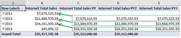
In this case we will be focused only on previous period calculations and to demonstrate DAX diversity here is an example how to get the same results using different functions and calculation techniques in DAX:

Internet Total Sales PY:=

CALCULATE (

    'Internet Sales'[Internet Total Sales],

    DATEADD ( 'Date'[Date], -1, YEAR )

)

Internet Total Sales PY2:=

CALCULATE (

    'Internet Sales'[Internet Total Sales],

    PARALLELPERIOD ( 'Date'[Date], -1, YEAR )

)

Internet Total Sales PY3:=

CALCULATE (

    'Internet Sales'[Internet Total Sales],

    PREVIOUSYEAR ( 'Date'[Date] )

)

In a given example DATEADD , PARALLELPERIOD and PREVIOUSYEAR will return the same result and they can be use interchangeably. Also, in certain cases they might be different based on dataset or on intermediate measures used, so the recommendation is to check the best option between these and test for desired results.

Requirements

Business requirement: Create one calculation and no matter which period of date hierarchy is selected return previous period. For example, if date is selected then return previous day, if month is selected then return month, etc. 

Problem: How to get individual time calculation for previous period from Date table and combine them together into one calculation due to fact that there is no unique calculation available in DAX for this task.

Date hierarchy: Year-Semester-Quarter-Month-Date

Solution:
As mentioned previously, there are several ways how to get individual period calculations working. In this case we will use DATEADD for function that will work for the most of our calculations.

Quick Solution

Previous day:

Internet Total Sales PD:=
CALCULATE (
    'Internet Sales'[Internet Total Sales],
    DATEADD ( 'Date'[Date], -1, DAY )
)

Previous month:
Internet Total Sales PM:=
CALCULATE (
    'Internet Sales'[Internet Total Sales],
    DATEADD ( 'Date'[Date], -1, MONTH )
)

Previous quarter:
Internet Total Sales PQ :=
CALCULATE (
    'Internet Sales'[Internet Total Sales],
    DATEADD ( 'Date'[Date], -1, QUARTER )
)

Calendar semester ID - calculated measure in Date table
Calendar Semester ID = ('Date'[Calendar Year] *100) + 'Date'[Calendar Semester]

Previous semester ID - Helper measure in Date table to accommodate MAX function which normally doesn't work with dates and strings:

Previous Semester ID:=

CALCULATE (

    MAX ( 'Date'[Calendar Semester ID] ),

    DATEADD ( 'Date'[Date], -6, MONTH )

)

Internet Total Sales Semester:

Internet Total Sales Semester:=
CALCULATE (
    'Internet Sales'[Internet Total Sales],
    FILTER (
        ALL ( 'Date' ),
        'Date'[Calendar Semester ID] = MAX('Date'[Calendar Semester ID])
 )
)


Internet Total Sales Previous Semester:
Internet Total Sales PS:=
CALCULATE (
    'Internet Sales'[Internet Total Sales Semester],
    PARALLELPERIOD ( 'Date'[Date], -6, MONTH )
)

Internet Total Sales Previous Year:
Internet Total Sales PY:=
CALCULATE (
    'Internet Sales'[Internet Total Sales],
    DATEADD ( 'Date'[Date], -1, YEAR )
)

Calendar Level Selected - Created test measure in Date dimension to check which level of hierarchy is selected:

Calendar Level Selected:=

SWITCH (

    TRUE (),

    HASONEVALUE ( 'Date'[Date] ), "Date selected",

    HASONEVALUE ( 'Date'[Month Calendar] ), "Month selected",

    HASONEVALUE ( 'Date'[Calendar Quarter] ), "Quarter selected",

    HASONEVALUE ( 'Date'[Calendar Semester] ), "Semester selected",

    HASONEVALUE ( 'Date'[Calendar Year] ), "Year selected",

    BLANK ()

)

Internet Total Sales Previous Period:
Internet Total Sales Previous Period:=
SWITCH (
    TRUE (),
    HASONEVALUE ( 'Date'[Date] ), [Internet Total Sales PD],
    HASONEVALUE ( 'Date'[Month Calendar] ), [Internet Total Sales PM],
    HASONEVALUE ( 'Date'[Calendar Quarter] ), [Internet Total Sales PQ],
    HASONEVALUE ( 'Date'[Calendar Semester] ), [Internet Total Sales PS],
    HASONEVALUE ( 'Date'[Calendar Year] ), [Internet Total Sales PY],
    BLANK ()
)

Previous Period Calculation - Explained

Previous month

Previous month calculation is relatively simple to get and will follow the logic within the calculation from below: use Calculate function and do an offset for month before.

Internet Total Sales PM:=
CALCULATE (
    'Internet Sales'[Internet Total Sales],
    DATEADD ( 'Date'[Date], -1, MONTH )
)

All other levels of hierarchy except previous semester can be calculated in the same way by changing time frame parameter in DATEADD function. 

Previous Semester

There is more of work around semester because there is no built in function available for semester calculation. In this case, we need more calculation and here is one of the ways to get it in DAX:

1. Calendar Semester ID - calculated column in Date dimension to get numeric ID which will be used later in MAX function, which will not accept any of date or string inputs, but number parameters.
2. Previous Semester ID (Date table) - test measure to get previous semester by doing 6 months offset in the past and taking Semester ID for given output of previous filter.
3. Internet Total Semester - get previous period ID FILTER function: ALL ( 'Date' ) to take off the filter selection on currently selected semester, go over all date and find previous semester. 'Date'[Calendar Semester ID] = MAX('Date'[Calendar Semester ID]) - if Max is not specified, the comparison will go over all repeated rows in the table which is not allowed by DAX and it will report error because of scalar use, and that's why MAX will work bringing only distinctive values for comparison and in this context I like to think of MAX as current semester. 
4. Internet Total Sales - go back in time 6 months and for that current semester using [Internet Total Semester] measure. In this case, PARALLELPERIOD  has been used here instead of FILTER that we used before.

Calendar Semester ID = ('Date'[Calendar Year] *100) + 'Date'[Calendar Semester]

Previous Semester ID:=

CALCULATE (

    MAX ( 'Date'[Calendar Semester ID] ),

    DATEADD ( 'Date'[Date], -6, MONTH )

)

Internet Total Sales Semester:=
CALCULATE (
    'Internet Sales'[Internet Total Sales],
    FILTER (
        ALL ( 'Date' ),
        'Date'[Calendar Semester ID] = MAX('Date'[Calendar Semester ID])
 )
)

Internet Total Sales PS:=
CALCULATE (
    'Internet Sales'[Internet Total Sales Semester],
    PARALLELPERIOD ( 'Date'[Date], -6, MONTH )
)

Combined Previous Period Calculation

After all of the hard work that we've done on individual calculation comes the challenge how to put them all together into one calculation.

Test Date Hierarchy Level Selected

The following example demonstrate how to recognize date hierarchy level based on filter selection. SWITCH which has been used here can be treated as multiple IF functions and HASONEVALUE will detect if certain period is selected either from filter selection or it's present in row context.

Calendar Level Selected:=

SWITCH (

    TRUE (),

    HASONEVALUE ( 'Date'[Date] ), "Date selected",

    HASONEVALUE ( 'Date'[Month Calendar] ), "Month selected",

    HASONEVALUE ( 'Date'[Calendar Quarter] ), "Quarter selected",

    HASONEVALUE ( 'Date'[Calendar Semester] ), "Semester selected",

    HASONEVALUE ( 'Date'[Calendar Year] ), "Year selected",

    BLANK ()

)

Previous Period Measure

Finally, based on all of the individual measures and switch function to detect date hierarchy levels that we've created earlier, we can easily get our combined previous period calculation.

Internet Total Sales Previous Period:=
SWITCH (
    TRUE (),
    HASONEVALUE ( 'Date'[Date] ), [Internet Total Sales PD],
    HASONEVALUE ( 'Date'[Month Calendar] ), [Internet Total Sales PM],
    HASONEVALUE ( 'Date'[Calendar Quarter] ), [Internet Total Sales PQ],
    HASONEVALUE ( 'Date'[Calendar Semester] ), [Internet Total Sales PS],
    HASONEVALUE ( 'Date'[Calendar Year] ), [Internet Total Sales PY],
    BLANK ()
)

SQL Reporting Services Tutorial (SSRS): T-SQL vs MDX vs DAX (with parameters)

SSRS Data Sources

SQL Reporting Services (SSRS) in all of its versions offers variety of data sources and different ways how to retrieve data from the source. In the examples following in this article I will be using SQL Server 2016 Developer Edition (RTM) which has these sources available:

• Microsoft SQL Server
• Microsoft Azure SQL Database
• Microsoft Analytics Platform System
• Microsoft SQL Server Analysis Services
• Microsoft SharePoint List
• Oracle Database
• Oracle Essbase
• SAP BW
• TERADATA
• OLEDB
• ODBC
• XML
• Report Server Model

SSRS in the nutshell uses different drivers to connect and pull data from the data source and as developers we are more interested in how to efficiently use them than knowing how they actually work. Another important layer in data retrieval is querying language which is specific to each of these data sources.
Our focus in this case will be SQL Server on both, Microsoft SQL Server and Microsoft SQL Server Analysis Services (SSAS). Also, we will be using 3 different languages to fetch the data from the 2 sources: T-SQL, MDX and DAX. 

The goal of this exercise is to get the same information using different querying languages from those 2 sources and to go through query basics and specifics for 3 of them as well as to learn how to build SSRS reports using parameters. 
Also, learning all 3 of them is from great benefit for every Microsoft BI full stack developer. Each of them can span from  basic data retrieval to complex queries or programing logic and definitely, they are worth of improving over time.

Sample data

Databases used here are taken from Microsoft samples currently available at github:

• Adventure Works Database (DW 2014) sample database
• Tabular Model Sample Database

Simple SSRS tutorials that I've created below will provide you enough of information to learn how to build some basic SSRS reports. In the most of cases, the report wizard has been used except for the queries which will be provided along with the exercises.

The final project (Visual Studio 2017 version) that I've developed as well as tutorials are available and can be downloaded from:
Visual Studio Project - SSRS using TSQL, MDX, DAX

Quick query comparison

The goal of this demonstration was to highlight 

• T- SQL - SQL Server Database Engine query language. 
• MDX - SSAS for both Tabular and multidimensional OLAP instances. Performance wise, it will be slower than DAX in tabular model, especially if tabular model contains  
• DAX - SSAS in Tabular model. It is still relatively new between the other 2 and probably, not intuitive for developers, but in syntax it is very similar to TSQL.

Probably, this could be another topic to compare the syntax of each language, but here is a quick snapshot for queries used in next sections:

T-SQL:

SELECT       

       pc.EnglishProductCategoryName AS CategoryName,

       ps.EnglishProductSubcategoryName AS SubCategoryName,

       p.EnglishProductName AS ProductName,

       SUM(s.SalesAmount) AS IntenetTotalSales,

    SUM(s.OrderQuantity) AS InternetTotalUnits

FROM FactInternetSales s

INNER JOIN DimProduct p

ON p.ProductKey = s.ProductKey

INNER JOIN DimProductSubcategory ps

ON ps.ProductSubcategoryKey = p.ProductSubcategoryKey

INNER JOIN DimProductCategory pc

ON pc.ProductCategoryKey = ps.ProductCategoryKey

INNER JOIN DimDate d

ON d.DateKey = s.OrderDateKey

INNER JOIN DimCustomer c

ON c.CustomerKey = s.CustomerKey

INNER JOIN DimGeography g

ON g.GeographyKey = c.GeographyKey

WHERE       

       d.CalendarYear = @pYear

       AND g.GeographyKey IN (SELECT GeographyKey FROM dbo.DimGeography where EnglishCountryRegionName =  @pCountryRegion)

GROUP BY pc.EnglishProductCategoryName, ps.EnglishProductSubcategoryName, p.EnglishProductName

ORDER BY CategoryName, SubCategoryName, ProductName

MDX:

SELECT

NON EMPTY {

       [Measures].[Internet Total Sales],

       [Measures].[Internet Total Units]

} ON COLUMNS,

NON EMPTY {

       (

       [Product Category].[Product Category Name].[Product Category Name].ALLMEMBERS *

       [Product Subcategory].[Product Subcategory Name].[Product Subcategory Name].ALLMEMBERS *

       [Product].[Product Name].[Product Name].ALLMEMBERS

       )

} ON ROWS

FROM [Adventure Works Internet Sales Model]

WHERE

(

       STRTOSET(@pYear, CONSTRAINED),

       STRTOSET(@pCountryRegion, CONSTRAINED)

)

DAX:

EVALUATE
 (
    FILTER (
        SUMMARIZE (
            'Internet Sales',
            'Product'[Product Category Name],
            'Product'[Product Subcategory Name],
            'Product'[Product Name],
            'Date'[Calendar Year],
            Geography[Country Region Name],
            "Internet Total Sales", [Internet Total Sales],
            "Internet Total Units", [Internet Total Units]
        ),
        'Date'[Calendar Year] = @pYear
            && Geography[Country Region Name] = @pCountryRegion
    )
)
ORDER BY
    'Product'[Product Category Name],
    'Product'[Product Subcategory Name],
    'Product'[Product Name]

SQL Server data source and T-SQL

Transaction SQL (T-SQL) is definitely, the most popular and probably, still the most used between the other 2 and it's dedicated to only relational SQL Database.


Here it goes, step by step tutorial:

1. Add new data source:

2. Create report (using report wizard):

**script used in the following section:

SELECT       

       pc.EnglishProductCategoryName AS CategoryName,

       ps.EnglishProductSubcategoryName AS SubCategoryName,

       p.EnglishProductName AS ProductName,

       SUM(s.SalesAmount) AS IntenetTotalSales,

    SUM(s.OrderQuantity) AS InternetTotalUnits

FROM FactInternetSales s

INNER JOIN DimProduct p

ON p.ProductKey = s.ProductKey

INNER JOIN DimProductSubcategory ps

ON ps.ProductSubcategoryKey = p.ProductSubcategoryKey

INNER JOIN DimProductCategory pc

ON pc.ProductCategoryKey = ps.ProductCategoryKey

INNER JOIN DimDate d

ON d.DateKey = s.OrderDateKey

INNER JOIN DimCustomer c

ON c.CustomerKey = s.CustomerKey

INNER JOIN DimGeography g

ON g.GeographyKey = c.GeographyKey

WHERE       

       d.CalendarYear = @pYear

       AND g.GeographyKey IN (SELECT GeographyKey FROM dbo.DimGeography where EnglishCountryRegionName =  @pCountryRegion)

GROUP BY pc.EnglishProductCategoryName, ps.EnglishProductSubcategoryName, p.EnglishProductName

ORDER BY CategoryName, SubCategoryName, ProductName

3. Rename main dataset:

4. Add year and country region datasets:


**script used in the following section:

SELECT

       DISTINCT

       CalendarYear

FROM dbo.DimDate

ORDER BY CalendarYear

**script used in the following section:

SELECT

       DISTINCT

       EnglishCountryRegionName as CountryRegion

FROM dbo.DimGeography

5. Bind year and country region datasets to parameters:

6. Slight formatting to the report (settings not explained here, but available in the project attached above):

SQL Server Analysis Services (Tabular model) source and MDX

Multidemnsional Expressions is a query language used against Online Analytical Processing (OLAP) and it can be ran against both, multidimensional and tabular instances of SSAS.



1. Add new data source:

2. Create report (using report wizard):

**script used in the following section:

SELECT

NON EMPTY {

       [Measures].[Internet Total Sales],

       [Measures].[Internet Total Units]

} ON COLUMNS,

NON EMPTY {

       (

       [Product Category].[Product Category Name].[Product Category Name].ALLMEMBERS *

       [Product Subcategory].[Product Subcategory Name].[Product Subcategory Name].ALLMEMBERS *

       [Product].[Product Name].[Product Name].ALLMEMBERS

       )

} ON ROWS

FROM [Adventure Works Internet Sales Model]

WHERE

(

       STRTOSET(@pYear, CONSTRAINED),

       STRTOSET(@pCountryRegion, CONSTRAINED)

)

3. Rename main parameters:

4. Rename main dataset:

5. Unhide parameters and review datasets:

6. Format report (settings not detailed here, but available in the project attached above) and review results:

SQL Server Analysis Services (Tabular model) source and DAX

Data Analytics Expressions is both, formula language and querying language dedicated only to tabular model instance of OLAP.

**data source "AdventureWorksTabular" already created in previous tutorials

1. Create report:

**script used in the following section:
EVALUATE
 (
    FILTER (
        SUMMARIZE (
            'Internet Sales',
            'Product'[Product Category Name],
            'Product'[Product Subcategory Name],
            'Product'[Product Name],
            'Date'[Calendar Year],
            Geography[Country Region Name],
            "Internet Total Sales", [Internet Total Sales],
            "Internet Total Units", [Internet Total Units]
        ),
        'Date'[Calendar Year] = @pYear
            && Geography[Country Region Name] = @pCountryRegion
    )
)
ORDER BY
    'Product'[Product Category Name],
    'Product'[Product Subcategory Name],
    'Product'[Product Name]

2. Rename main dataset:

3. Create year and region country datasets (to be consumed in parameters):

**script used in the following section:
EVALUATE
(
    SUMMARIZE(
        'Date',
        'Date'[Calendar Year]
    )
)
ORDER BY
    'Date'[Calendar Year]

**script used in the following section:
EVALUATE
(
    SUMMARIZE(
        'Geography',
        Geography[Country Region Name]
    )
)
ORDER BY
    Geography[Country Region Name]

4. Bind datasets to parameters:

5. Format report (settings not detailed here, but available in the project attached above) and review results: